PID Visualizer

Project Overview

Because I use PIDs frequently in robotics, I made a visualization of how a PID works to make it easier to understand. I'll explain what PIDs are and how they work, as well as show off my visualization. As a bonus, at the end, I'll discuss how to improve your PIDs by using a trapezoidal motion profile.

The code shown here has been modified to make it easier to explain. If you would like to check it out, the full code is available on GitHub: PID Visualizer

What is a PID and Where is it Used?

PID, or proportional integral derivative, is a control algorithm. It is a technique for getting value A to become value B while accounting for acceleration and inertia. We can see this in action by looking at a graph of a PID output:

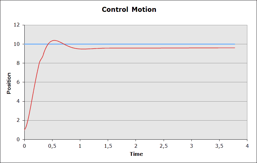
The blue line represents the target, while the red line represents the PID algorithm's output. The PID output begins slowly and then accelerates. In the end, the PID progressively slows down to accommodate for inertia. PIDs are very configurable; you can tweak a PID to arrive at the destination as rapidly as possible, as precisely as possible, or a combination of the two.

PIDs are utilized everywhere, including in your home and automobile. They are used in houses to keep the temperature stable, and they are utilized in your automobile to maintain a certain speed using cruise control. PIDs are everywhere, regulating everything you use.

How PID Works

First, let's define some terms:

• Actual: The present location of your output (for example, the position of a robotic arm, the speed of a car, the temperature of a room, and so on).
• Setpoint: The desired location of your output.
• Error: 'Setpoint - Actual' The difference between your current location and your desired location

Next, let's look at the equation for a PID and break each part down:

Proportional Term (P):

The proportional term is calculated by multiplying the error by a constant kP. kP is determined by starting with a random number (typically a factor of 10 less than 1) and changing it until you get the outcome you want. There are a few mathematical methods for tuning a PID, but because of the vast variety of possible "solutions," it is typically best to adjust it by hand. The proportional term has the greatest overall influence on the PID output.

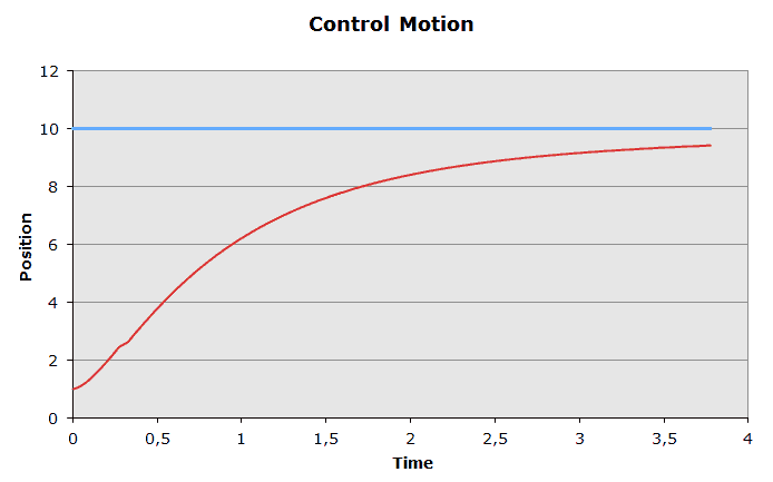
• To low of a kP term

Integral Term (I):

The integral term is calculated by integrating over all errors since the start of the PID and multiplying it by a constant kI. kI is normally a relatively small number since a large kI can cause oscillation. Because of these problems, the integral term is often restricted to a small value. The integral term is a push to get the actual to the setpoint.

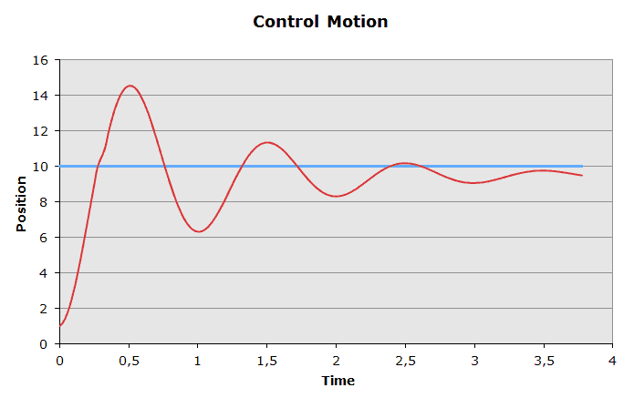
• Here you can see oscillation within a PID, probably too high of a kI

Derivative Term (D):

Taking the derivative of the error with regard to time multiplied by kD yields the derivative term. When attempting to account for external factors, the term can be beneficial. It helps to soften large, abrupt changes in error. The derivative term can cancel out events such as a car on cruise control suddenly going down a slope or a block of ice being placed in a room that is trying to keep a consistent temperature.

Tuning a PID

I mentioned it previously, but let me go over how to tune a PID. Because each PID has particular requirements, the best approach is to adjust the constants until you get an output you like. I suggest beginning with the kP term, then tweaking kI, and finally kD. You might find that you don't need the D or I constants at all. Some applications require simply P, PI, or PD. I've never seen it used before, but I'm sure you could find an application for ID.

PID Visualizer

Here's a simulation of a PID I created to showcase how it works:

The slider adjusts the PID's setpoint. You can modify kP, kI, and kD to get different PID outputs.

BONUS Taking PID to the Next Level

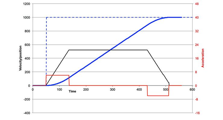
PIDs are a complex method of modeling motion but break down in complex real-world situations. With trapezoidal motion profiles, we can model more complex motion and account for many more factors. Trapezoidal motion profiles work by first calculating a theoretically perfect path to get A to become B using a given maximum velocity and maximum acceleration.

To get from this path to motor output, we need to do some math:

• p(t) = position over time | v(t) = velocity over time | a(t) = acceleration over time
• S term is in the direction of v(t)
• G term will vary depending on the object

We start with the velocity term, which is the predicted velocity multiplied by a constant kV. The velocity term is the largest factor in the movement of the object. Next, we have the acceleration term, which is similar to the velocity term but with predicted acceleration and kA. This term is active at the beginning and end of a motion and helps with acceleration and deceleration. After that, we have the gravitational term. The job of the gravitational term is to counteract the forces of gravity, which are different for every application, so there is no one equation for it. Commonly the gradational term is represented by the cosine of the position as when the cosine is the largest, so are the gradational forces. Finally, we have the “S” term, which is used to account for all friction in the system. Because the friction is related to the direction of the velocity, the “S” term is multiplied by the sign of the velocity.

Additionally, you can add a PID between the current position and the predicted position to make sure the object follows the motion profile with greater accuracy. This can also be helpful in accounting for spring back when the object comes to a stop.

Full code: PID Visualizer

Images from:

• https://jjrobots.com/pid/
• https://www.motioncontroltips.com/what-is-a-motion-profile/